Static maps
mapping.RdFunction to produce static maps from an object of class sf, IT, EU, US, or WR.
Usage
mapping(data = NULL, var = NULL, colID = NULL,
type = c("static", "interactive"),
typeStatic = c("tmap", "choro.cart", "typo","bar"),
add_text = NULL, subset = NULL, facets = NULL, aggregation_fun = sum,
aggregation_unit = NULL, options = mapping.options(), ...)Arguments
- data
an object of class
sf,IT,EU,US, orWR- var
character value(s) or columns number(s) indicating the variable to plot
- colID
character value or columns number indicating the column with unit names
- type
if generates static or interactive map
- typeStatic
type of static map
- add_text
character name indicating the column with text labels
- subset
a formula indicating the condition to subset the data. See the details
- facets
variable(s) name to split the data
- aggregation_fun
function to use when data are aggregated
- aggregation_unit
variable name by which the unit are aggregate
- options
a list with options using
mapping.optionsfunction- ...
further arguments
Details
It is a general function to map data. We can externally provide the coordinates with the variable to map, or the coordinates and the data to link.
If coordinates are provided and data is NULL, the function map the var in coordinates. If data is not NULL, then the function link data and coordinates, and the var is get from the data provided in input.
If only data are provided without coordinates, the function search the colID among the the coordinates dataset provided by https://github.com/mappinguniverse/geospatial, to link the ids with coordinates. For search look at SearchNames
References
Giraud, T. and Lambert, N. (2016). cartography: Create and Integrate Maps in your R Workflow. JOSS, 1(4). doi: 10.21105/joss.00054.
Pebesma, E., 2018. Simple Features for R: Standardized Support for Spatial Vector Data. The R Journal 10 (1), 439-446, https://doi.org/10.32614/RJ-2018-009
Tennekes M (2018). “tmap: Thematic Maps in R.” _Journalstatisticaltical Software_, *84*(6), 1-39. doi: 10.18637/jss.v084.i06 (URL: https://doi.org/10.18637/jss.v084.i06).
Examples
library(dplyr)
#>
#> Attaching package: ‘dplyr’
#> The following objects are masked from ‘package:stats’:
#>
#> filter, lag
#> The following objects are masked from ‘package:base’:
#>
#> intersect, setdiff, setequal, union
library(sf)
#> Linking to GEOS 3.10.2, GDAL 3.4.1, PROJ 8.2.1; sf_use_s2() is TRUE
data("popIT")
popIT <- popIT
coords <- loadCoordIT(unit = "provincia", year = '2019')
cr <- left_join(coords, popIT, by = c( "provincia" = "ID"))
###############
# Statics #
###############
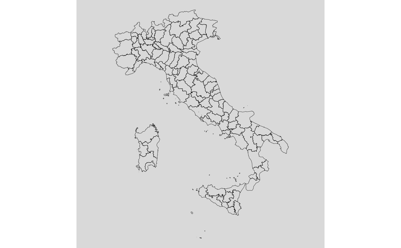
mapping(cr)
 # \donttest{
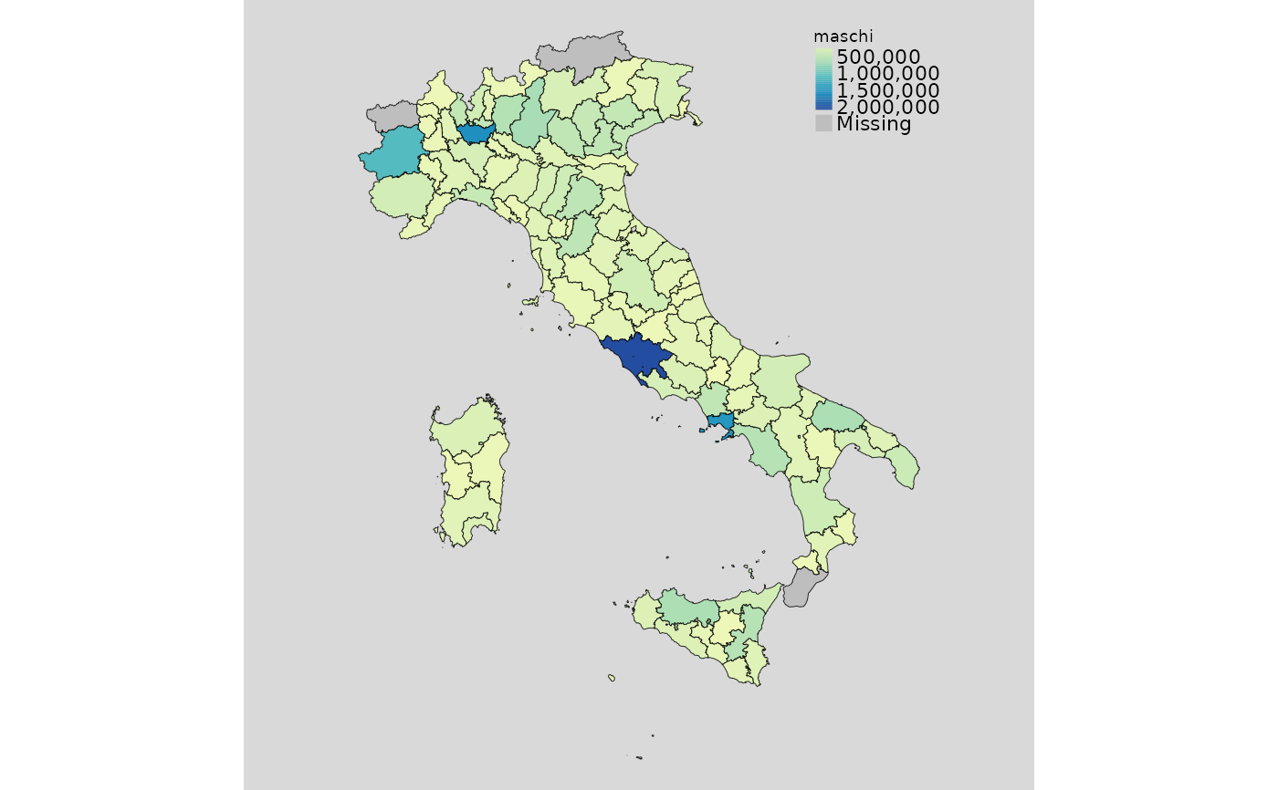
mapping(cr, var = "maschi")
# \donttest{
mapping(cr, var = "maschi")
 nc = st_read(system.file("shape/nc.shp", package="sf"))
#> Reading layer `nc' from data source
#> `/home/runner/work/_temp/Library/sf/shape/nc.shp' using driver `ESRI Shapefile'
#> Simple feature collection with 100 features and 14 fields
#> Geometry type: MULTIPOLYGON
#> Dimension: XY
#> Bounding box: xmin: -84.32385 ymin: 33.88199 xmax: -75.45698 ymax: 36.58965
#> Geodetic CRS: NAD27
class(nc)
#> [1] "sf" "data.frame"
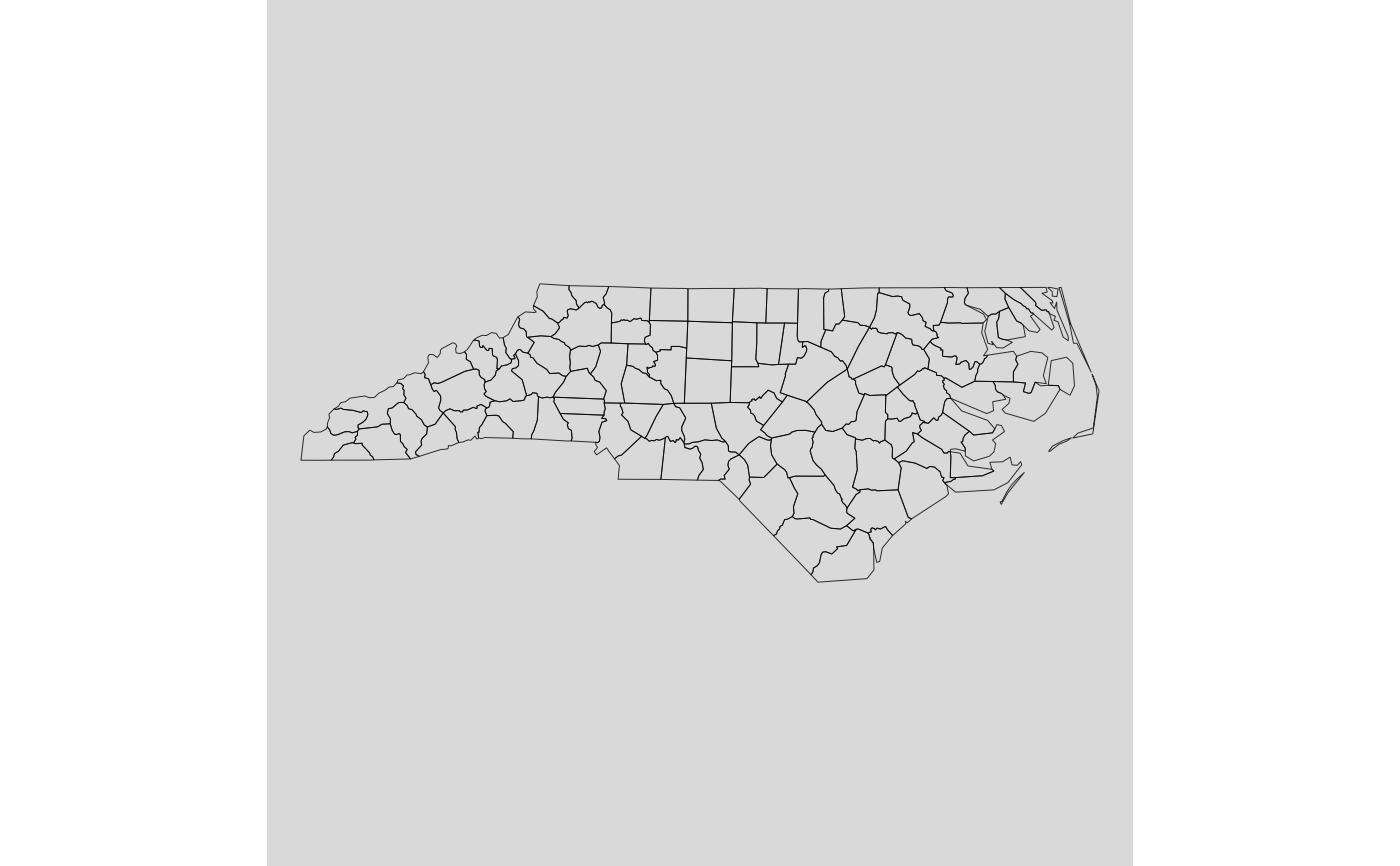
mapping(nc)
nc = st_read(system.file("shape/nc.shp", package="sf"))
#> Reading layer `nc' from data source
#> `/home/runner/work/_temp/Library/sf/shape/nc.shp' using driver `ESRI Shapefile'
#> Simple feature collection with 100 features and 14 fields
#> Geometry type: MULTIPOLYGON
#> Dimension: XY
#> Bounding box: xmin: -84.32385 ymin: 33.88199 xmax: -75.45698 ymax: 36.58965
#> Geodetic CRS: NAD27
class(nc)
#> [1] "sf" "data.frame"
mapping(nc)
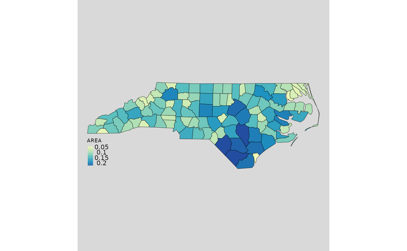
 mapping(nc, var = "AREA", options = mapping.options(legend.position = c("left", "bottom")))
 ###############
# Interactive #
###############
mapping(cr, type = "interactive")
mapping(cr, var = "maschi", type = "interactive")
nc = st_read(system.file("shape/nc.shp", package="sf"))
#> Reading layer `nc' from data source
#> `/home/runner/work/_temp/Library/sf/shape/nc.shp' using driver `ESRI Shapefile'
#> Simple feature collection with 100 features and 14 fields
#> Geometry type: MULTIPOLYGON
#> Dimension: XY
#> Bounding box: xmin: -84.32385 ymin: 33.88199 xmax: -75.45698 ymax: 36.58965
#> Geodetic CRS: NAD27
class(nc)
#> [1] "sf" "data.frame"
mapping(nc, type = "interactive")
mapping(nc, var = "AREA", type = "interactive")
# }
###############
# Interactive #
###############
mapping(cr, type = "interactive")
mapping(cr, var = "maschi", type = "interactive")
nc = st_read(system.file("shape/nc.shp", package="sf"))
#> Reading layer `nc' from data source
#> `/home/runner/work/_temp/Library/sf/shape/nc.shp' using driver `ESRI Shapefile'
#> Simple feature collection with 100 features and 14 fields
#> Geometry type: MULTIPOLYGON
#> Dimension: XY
#> Bounding box: xmin: -84.32385 ymin: 33.88199 xmax: -75.45698 ymax: 36.58965
#> Geodetic CRS: NAD27
class(nc)
#> [1] "sf" "data.frame"
mapping(nc, type = "interactive")
mapping(nc, var = "AREA", type = "interactive")
# }