Introduction
mapping allows to easily show data using maps, without concern about the geographical coordinates which are provided in the package and automatically link with the data. The mapping functions use the already available and well implemented function in tmap, cartography, and leaflet packages.
Since different countries have different geographical structure, and, in particular, different statistical unit or different subdivision, mapping provide a single function for static and interactive plots of such subvisions:
| Country | Function Static |
|---|---|
| World | mappingWR() |
| European Union | mappingEU() |
| Italy | mappingIT() |
| United States of America | mappingUS() |
In addition a generic mapping() function is also
provided, and explained in a specific section.
The most important step is to link each country, partition or statistical unit with their coordinates. The package also provides specific function to automatically build a object with data and coordinates:
| Coordinates | Function | Object Class |
|---|---|---|
| World | WR() |
WR |
| European Union | EU() |
EU |
| Italy | IT() |
IT |
| United States of America | US() |
US |
The data can be linked first building the object with its specific
function or using the mapping function which automatically
will both link, and then map the input data.
The CRAN version can be loaded as follows:
or the development version from GitHub:
remotes::install_github('serafinialessio/mapping')The population data, available in the package, will be used to describe the package features
data("popWR")
str(popWR)
## 'data.frame':    269 obs. of  5 variables:
##  $ country     : Factor w/ 265 levels "","Afghanistan",..: 2 3 4 5 6 7 8 10 11 12 ...
##  $ country_code: Factor w/ 265 levels "","ABW","AFG",..: 3 5 60 11 6 4 12 9 10 2 ...
##  $ total       : num  37172386 2866376 42228429 55465 77006 ...
##  $ male        : num  19093281 1460043 21332000 NA NA ...
##  $ female      : num  18079105 1406333 20896429 NA NA ...
data("popEU")
str(popEU)
## 'data.frame':    2252 obs. of  5 variables:
##  $ TIME  : num  2019 2019 2019 2019 2019 ...
##  $ GEO   : chr  "BE" "BE1" "BE10" "BE100" ...
##  $ total : num  11455519 1215290 1215290 1215290 6596233 ...
##  $ male  : num  5644826 597008 597008 597008 3265134 ...
##  $ female: num  5810693 618282 618282 618282 3331099 ...
data("popIT")
str(popIT)
## 'data.frame':    107 obs. of  4 variables:
##  $ ID     : chr  "Roma" "Milano" "Napoli" "Torino" ...
##  $ maschi : num  2081239 1576316 1497289 1092504 624201 ...
##  $ femmine: num  2260973 1673999 1587601 1167019 641753 ...
## $ totale : num 4342212 3250315 3084890 2259523 1265954 ...Load coordinates and check names
Coordinates can be separately downloaded using this specific functions
| Coordinates | Function |
|---|---|
| World | loadCoordWR() |
| European Union | loadCoordEU() |
| Italy | loadCoordIT() |
| United States of America | loadCoordUS() |
Coordinates are download from the GitHub repository , which provides
.geojson and .RData files with coordinates, which return an object of
class sf.
coord_eu <- loadCoordEU(unit = "nuts0")The unit argument in the load functions,
indicates the type of statistical unit, geographical subdivision or
level of aggregation, which is specific for the country. For example, in
this case, the EU has different statistical units, and we are interested
to get coordinates for “nuts0”, i.e. for European countries.
library(tmap)
tm_shape(coord_eu) + tm_borders()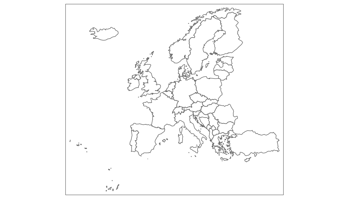
Returning an object of class sf, we can also use the
mapping function available in the other R packages.
Note that, the data are downloaded from an online repository, and
then an internet connection should be preferred. Nevertheless, if the
use_internet argument set to FALSE, we will
get the coordinates locally available in the package.
The names provided from the user, and the names available in the
package have to be the same to link the coordinate.
checkNames functions will return the nomatching names:
checkNamesIT(popIT$ID, unit = "provincia")
## [1] "reggio di calabria"             "bolzano / bozen"
## [3] "valle d'aosta / vallée d'aoste"
GetNames functions returns the names used in the
packages for each unit.
getNamesEU(unit = "nuts0")
##                                                 country iso2 iso3 country_code
## 1                                               Germany   DE  DEU          276
## 2                                               Czechia   CZ  CZE          203
## 3                                              Bulgaria   BG  BGR          100
## 4                                           Switzerland   CH  CHE          756
## 5                                               Albania   AL  ALB            8
## 6                                               Austria   AT  AUT           40
## 7                                                Cyprus   CY  CYP          196
## 8                                                Greece   GR  GRC          300
## 9                                               Belgium   BE  BEL           56
## 10                                               France   FR  FRA          250
## 11                                              Denmark   DK  DNK          208
## 12                                              Estonia   EE  EST          233
## 13                                                Spain   ES  ESP          724
## 14                                              Finland   FI  FIN          246
## 15                                               Norway   NO  NOR          578
## 16                                               Sweden   SE  SWE          752
## 17                                             Slovenia   SI  SVN          705
## 18                                          Netherlands   NL  NLD          528
## 19                                                Italy   IT  ITA          380
## 20                                            Lithuania   LT  LTU          440
## 21                                           Luxembourg   LU  LUX          442
## 22                                               Latvia   LV  LVA          428
## 23                                           Montenegro   ME  MNE          499
## 24                                      North Macedonia   MK  MKD          807
## 25                                                Malta   MT  MLT          470
## 26                                              Romania   RO  ROU          642
## 27                                               Serbia   RS  SRB          688
## 28                                              Croatia   HR  HRV          191
## 29                                             Slovakia   SK  SVK          703
## 30                                        Liechtenstein   LI  LIE          438
## 31                                             Portugal   PT  PRT          620
## 32                                              Hungary   HU  HUN          348
## 33                                              Ireland   IE  IRL          372
## 34                                              Iceland   IS  ISL          352
## 35 United Kingdom of Great Britain and Northern Ireland   GB  GBR          826
## 36                                               Poland   PL  POL          616
## 37                                               Turkey   TR  TUR          792
##    nuts0_id                                                nuts0
## 1        DE                                              Germany
## 2        CZ                                              Czechia
## 3        BG                                             Bulgaria
## 4        CH                                          Switzerland
## 5        AL                                              Albania
## 6        AT                                              Austria
## 7        CY                                               Cyprus
## 8        EL                                               Greece
## 9        BE                                              Belgium
## 10       FR                                               France
## 11       DK                                              Denmark
## 12       EE                                              Estonia
## 13       ES                                                Spain
## 14       FI                                              Finland
## 15       NO                                               Norway
## 16       SE                                               Sweden
## 17       SI                                             Slovenia
## 18       NL                                          Netherlands
## 19       IT                                                Italy
## 20       LT                                            Lithuania
## 21       LU                                           Luxembourg
## 22       LV                                               Latvia
## 23       ME                                           Montenegro
## 24       MK                                      North Macedonia
## 25       MT                                                Malta
## 26       RO                                              Romania
## 27       RS                                               Serbia
## 28       HR                                              Croatia
## 29       SK                                             Slovakia
## 30       LI                                        Liechtenstein
## 31       PT                                             Portugal
## 32       HU                                              Hungary
## 33       IE                                              Ireland
## 34       IS                                              Iceland
## 35       UK United Kingdom of Great Britain and Northern Ireland
## 36       PL                                               Poland
## 37       TR                                               Turkey
getNamesEU(unit = "nuts0", all_levels = FALSE)
##  [1] Germany
##  [2] Czechia
##  [3] Bulgaria
##  [4] Switzerland
##  [5] Albania
##  [6] Austria
##  [7] Cyprus
##  [8] Greece
##  [9] Belgium
## [10] France
## [11] Denmark
## [12] Estonia
## [13] Spain
## [14] Finland
## [15] Norway
## [16] Sweden
## [17] Slovenia
## [18] Netherlands
## [19] Italy
## [20] Lithuania
## [21] Luxembourg
## [22] Latvia
## [23] Montenegro
## [24] North Macedonia
## [25] Malta
## [26] Romania
## [27] Serbia
## [28] Croatia
## [29] Slovakia
## [30] Liechtenstein
## [31] Portugal
## [32] Hungary
## [33] Ireland
## [34] Iceland
## [35] United Kingdom of Great Britain and Northern Ireland
## [36] Poland
## [37] Turkey
## 37 Levels: Albania Austria Belgium Bulgaria Croatia Cyprus Czechia ... United Kingdom of Great Britain and Northern Ireland
Building a mapping object
Before building a map of our data, we have to link the
ids with coordinates, which is automatic in
mapping package using specific functions:
| Coordinates | Function | Object Class |
|---|---|---|
| World | WR() |
WR |
| European Union | EU() |
EU |
| Italy | IT() |
IT |
| United States of America | US() |
US |
These are the functions to build the dataset with data and coordinates, and, using specific arguments, we can manipulate the data before mapping.
The popIT, as showed in the previous section, does not
contain any information about the geographical geometries:
str(popIT)
## 'data.frame':    107 obs. of  4 variables:
##  $ ID     : chr  "Roma" "Milano" "Napoli" "Torino" ...
##  $ maschi : num  2081239 1576316 1497289 1092504 624201 ...
##  $ femmine: num  2260973 1673999 1587601 1167019 641753 ...
##  $ totale : num  4342212 3250315 3084890 2259523 1265954 ...
then, the coordinates are added as follows:
it <- IT(data = popIT, unit = "provincia", year = "2018",colID = "ID")We have to specify the type of statistical unit, the column containing the ids and, if necessary, the year of the subdivision. The functions will automatically download the coordinates linking them to the data. In this example, we have data about the population of the Italian province in 2018.
library(tmap)
tm_shape(it) + tm_borders() + tm_fill("totale")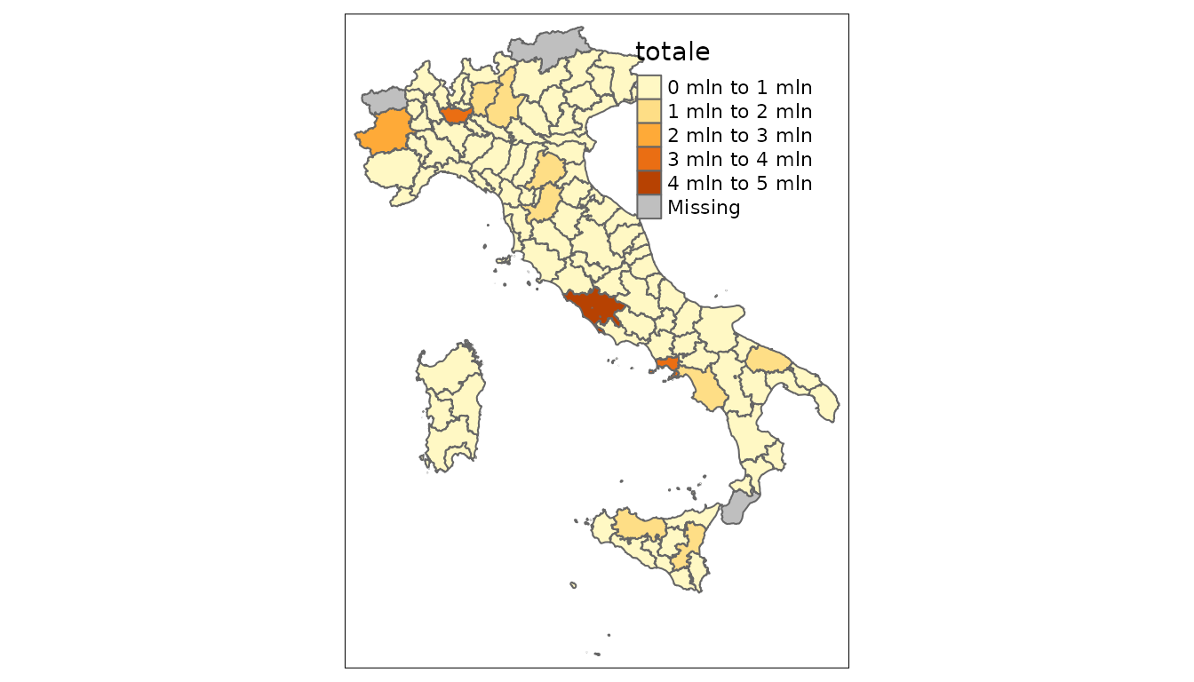
We have missing observation because the names in the data are different from the name in the package, as showed before.
The unit belongs to different levels of
aggregation/division. We can think at this as an hierarchy,
i.e. starting from a subdivision we can know all the larger aggregation
and then building the bigger geographical object.
This diagram shows an example of this hierarchy, with the largest level, level0, to the smaller, level4. If we have a level3 unit, we will have all the largest one until the level0.
In linking the data and the coordinates, the functions available in
this packages will return also the information about larger units. For
example, in the Italian case the it data will have a column
indicating the ripartizione and regione, which
are larger aggregates than provincia. Building the
hierarchy is available for all functions in this section and it is also
available in the loading functions.
str(it,1)
## Classes 'sf', 'IT', 'IT' and 'data.frame':   107 obs. of  11 variables:
##  $ ripartizione     : chr  "Nord-ovest" "Nord-ovest" "Nord-ovest" "Nord-ovest" ...
##  $ regione          : chr  "Piemonte" "Piemonte" "Piemonte" "Piemonte" ...
##  $ code_ripartizione: int  1 1 1 1 1 1 1 1 1 1 ...
##  $ code_regione     : int  1 1 1 1 1 1 2 7 7 7 ...
##  $ code_provincia   : int  1 2 3 4 5 6 7 8 9 10 ...
##  $ ID               : chr  "torino" "vercelli" "novara" "cuneo" ...
##  $ code             : chr  "TO" "VC" "NO" "CN" ...
##  $ maschi           : num  1092504 82848 179588 289459 105011 ...
##  $ femmine          : num  1167019 88063 189430 297639 109627 ...
##  $ totale           : num  2259523 170911 369018 587098 214638 ...
##  $ geometry         :sfc_MULTIPOLYGON of length 107; first list element: List of 1
##   ..- attr(*, "class")= chr [1:3] "XY" "MULTIPOLYGON" "sfg"
##  - attr(*, "sf_column")= chr "geometry"
##  - attr(*, "agr")= Factor w/ 3 levels "constant","aggregate",..: NA NA NA NA NA NA NA NA NA NA
##   ..- attr(*, "names")= chr [1:10] "ripartizione" "regione" "code_ripartizione" "code_regione" ...
##  - attr(*, "unit")= chr "provincia"
##  - attr(*, "year")= chr "2018"
##  - attr(*, "colID")= chr "ID"
Data can be subsets before mapping
it <- IT(data = popIT, unit = "provincia",
         year = "2018",colID = "ID",
         subset = ~ I(regione == "Lazio"))
in this case, we use the hierarchy to retrieve only the data of “Lazio” region.
library(tmap)
tm_shape(it) + tm_borders()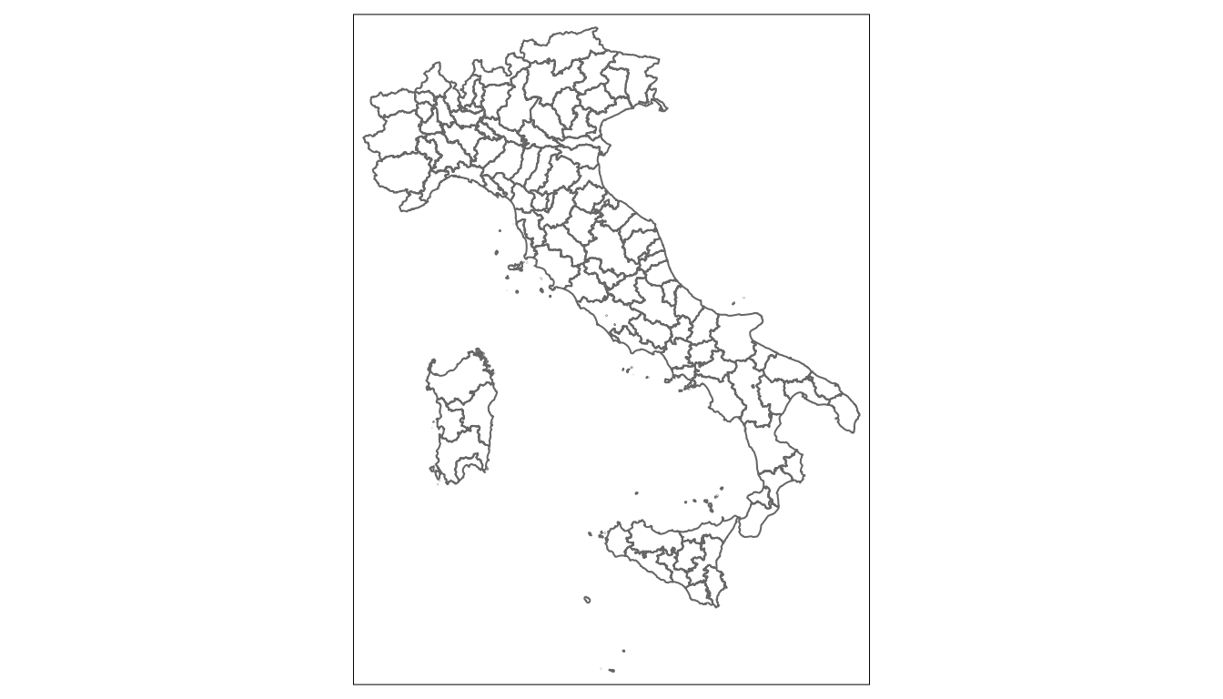
Suppose now to want the percentage of male and female, but we have only the total number:
it <- IT(data = popIT, unit = "provincia",
         year = "2018",colID = "ID",
         add = ~I(maschi/totale) + I(femmine/totale),
         new_var_names = c("Male percentage", "Female percentage"),
         print = FALSE)

str(it,1)
## Classes 'sf', 'IT', 'IT' and 'data.frame':   107 obs. of  13 variables:
##  $ ripartizione     : chr  "Nord-ovest" "Nord-ovest" "Nord-ovest" "Nord-ovest" ...
##  $ regione          : chr  "Piemonte" "Piemonte" "Piemonte" "Piemonte" ...
##  $ code_ripartizione: int  1 1 1 1 1 1 1 1 1 1 ...
##  $ code_regione     : int  1 1 1 1 1 1 2 7 7 7 ...
##  $ code_provincia   : int  1 2 3 4 5 6 7 8 9 10 ...
##  $ ID               : chr  "torino" "vercelli" "novara" "cuneo" ...
##  $ code             : chr  "TO" "VC" "NO" "CN" ...
##  $ maschi           : num  1092504 82848 179588 289459 105011 ...
##  $ femmine          : num  1167019 88063 189430 297639 109627 ...
##  $ totale           : num  2259523 170911 369018 587098 214638 ...
##  $ Male.percentage  : 'AsIs' num  0.483510.... 0.484743.... 0.486664.... 0.493033.... 0.489247.... ...
##  $ Female.percentage: 'AsIs' num  0.516489.... 0.515256.... 0.513335.... 0.506966.... 0.510752.... ...
##  $ geometry         :sfc_MULTIPOLYGON of length 107; first list element: List of 1
##   ..- attr(*, "class")= chr [1:3] "XY" "MULTIPOLYGON" "sfg"
##  - attr(*, "sf_column")= chr "geometry"
##  - attr(*, "agr")= Factor w/ 3 levels "constant","aggregate",..: NA NA NA NA NA NA NA NA NA NA ...
##   ..- attr(*, "names")= chr [1:12] "ripartizione" "regione" "code_ripartizione" "code_regione" ...
##  - attr(*, "unit")= chr "provincia"
##  - attr(*, "year")= chr "2018"
##  - attr(*, "colID")= chr "ID"
Now, we have now the percentage and we have named the new variables.
Note that, we can also build directly this object in the
mapping functions, but we can not manipulate the data and
build an unique object to be used in different mapping functions.
Countries ids or units may have different names. For example, we can
have a iso2 name instead of a formal name. The matchWith
argument indicates the type of names we have to link.
eu <- EU(data = popEU, unit = "nuts0", colID = "GEO",
         matchWith = "id", check.unit.names = FALSE)
The popEU data have nuts expressed with ids,
which is specified in the matchWith.
Static maps
We start with a map of the European Union countries
mappingEU(data = coord_eu)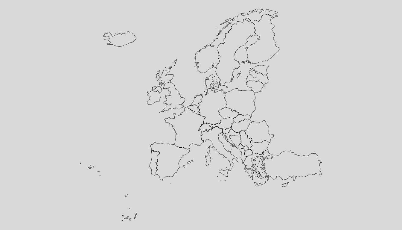
In this case, we do not provide any data to map. Now, we suppose to want to look at the distribution of population among European countries
eu <- EU(data = popEU, unit = "nuts0", colID = "GEO",
         matchWith = "iso2", check.unit.names = FALSE)
mappingEU(eu, var = "total")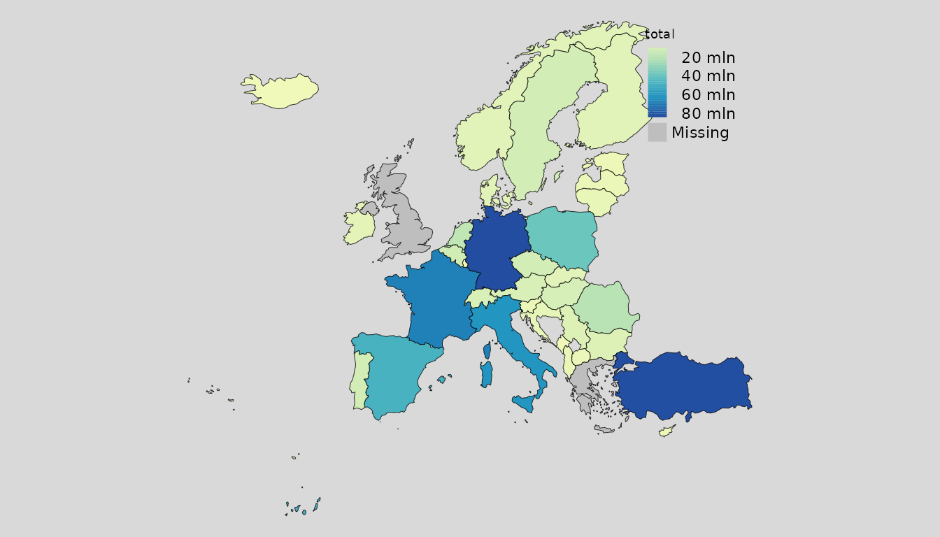
where, matchWith is equal to “iso2” because the id name
in popEU are expressed according to iso2 code, instead of
iso3 or country names.
It is equivalent to use mapping function without building as
EU object
mappingEU(data = popEU,unit = "nuts0", colID = "GEO", matchWith = "iso2", var = "total")
Of course, the mapping function provides arguments to work and modify data before mapping.
The loadCoord functions, as explained in the previous
section, automatically return all the bigger statistical unit
aggregation. We can easily use this in mapping functions, in which the
value of the variables are sum for each
aggragation_unit
eu <- EU(data = popEU, unit = "nuts1", colID = "GEO",
         matchWith = "id", check.unit.names = FALSE)
mappingEU(eu, var = "total")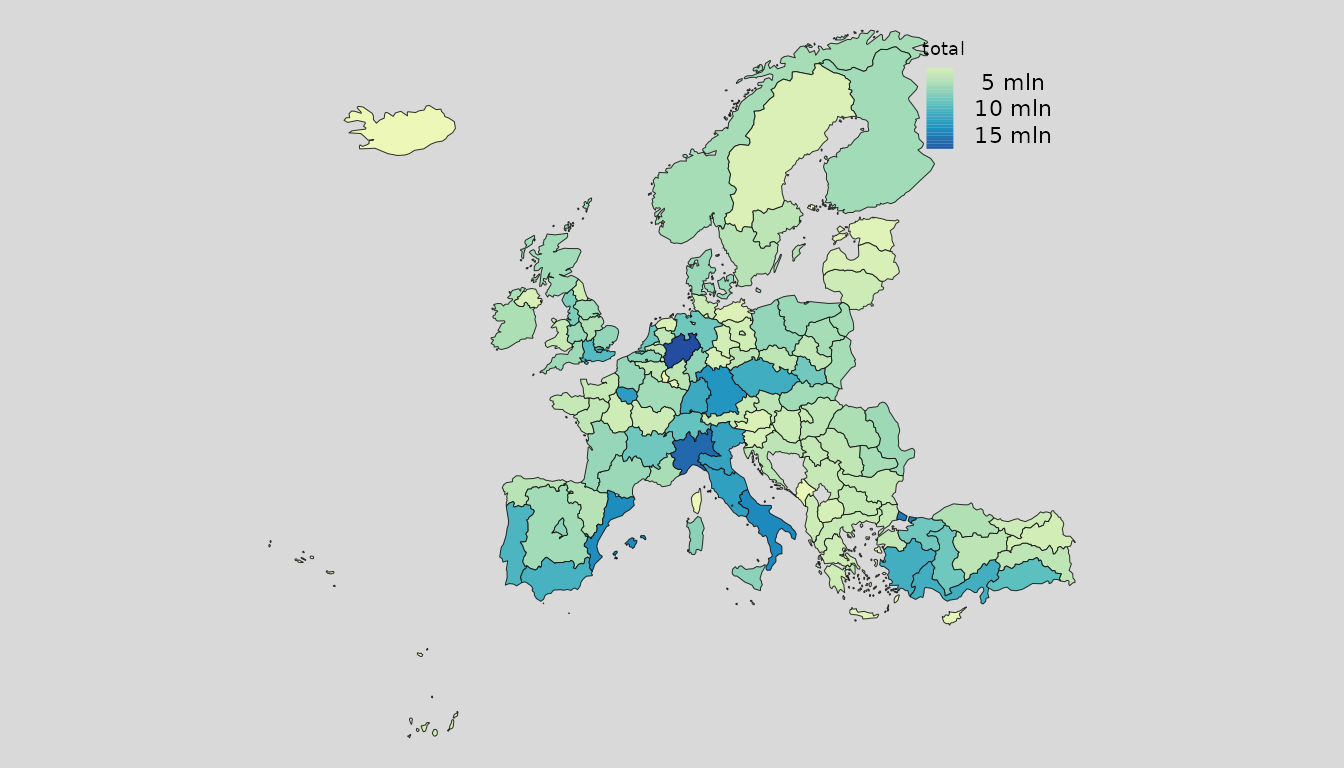
mappingEU(eu, var = "total", aggregation_unit = "nuts0", aggregation_fun = sum)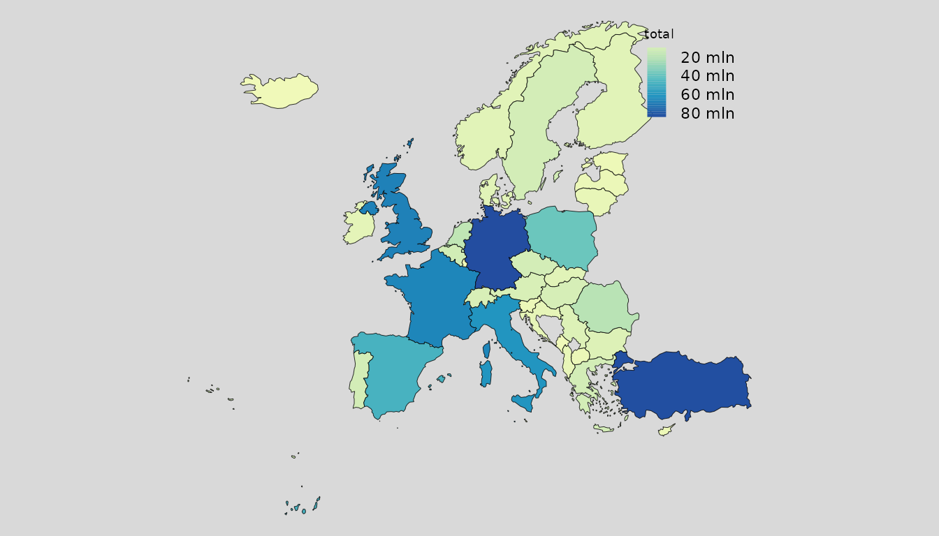
We can also provide multiple variables to generate multiple maps
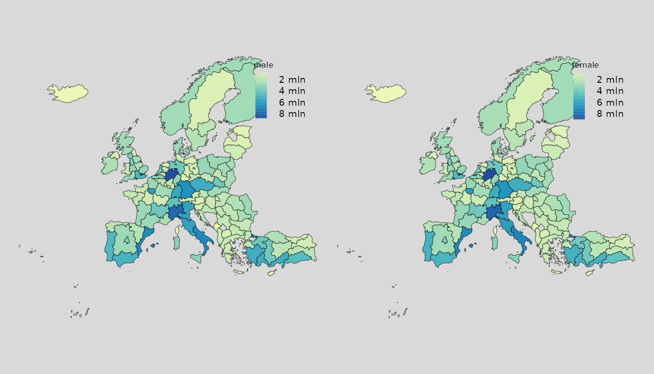
or, if we are not interested in the entire data but in a specific subset, we can apply a subset statement before mapping
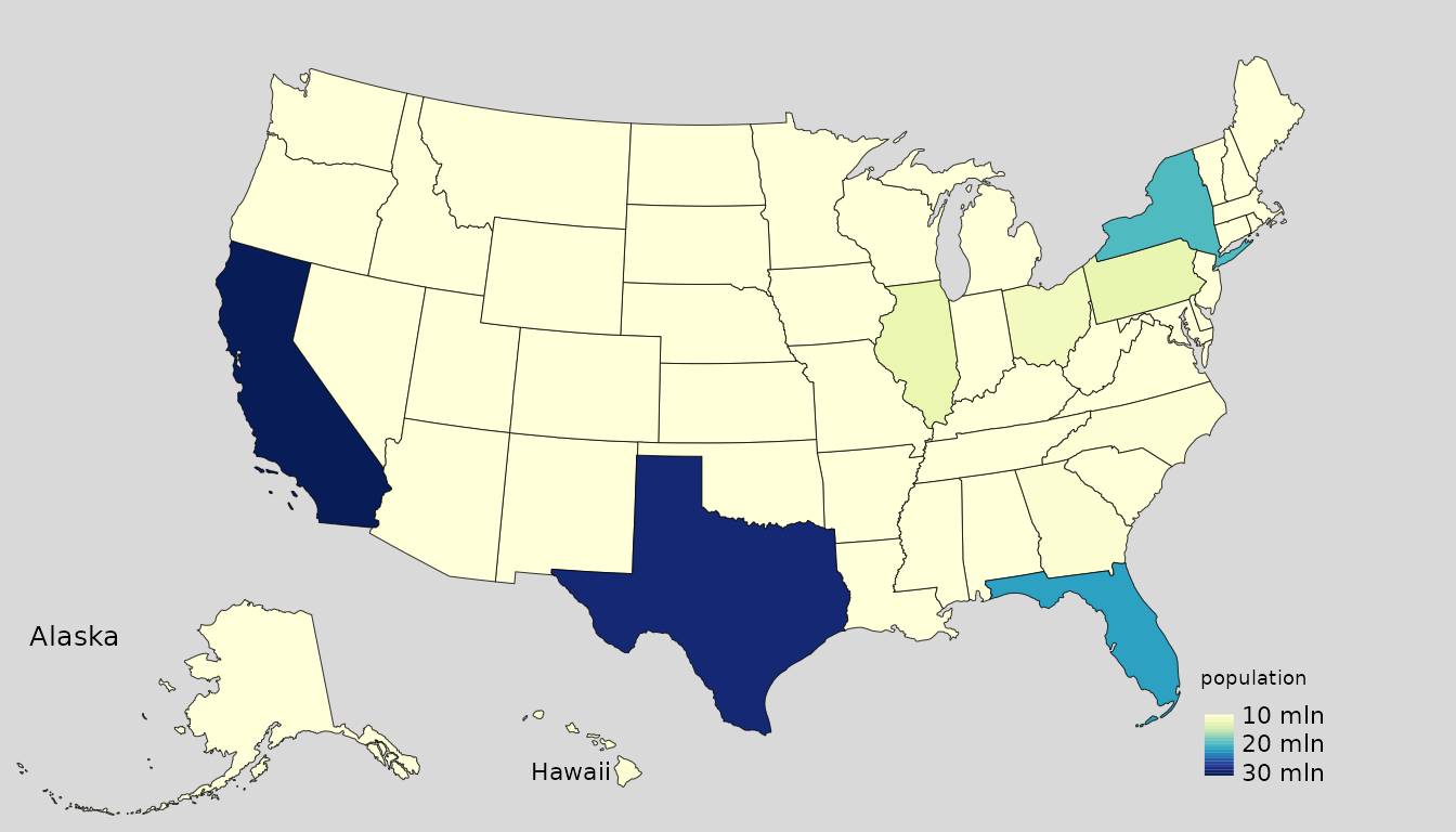
Let’s look at USA example.
mappingUS(us, var = "population")
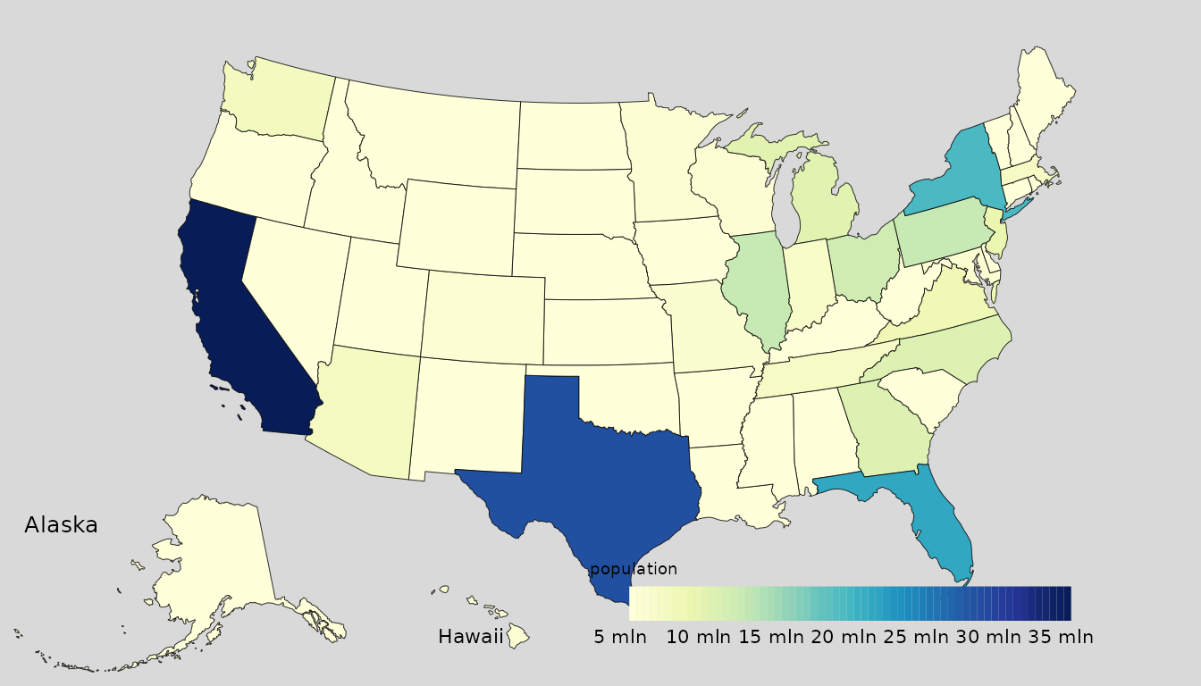
mappingUS(us, var = "population", options = mapping.options(nclass = 10, legend.portrait = FALSE))
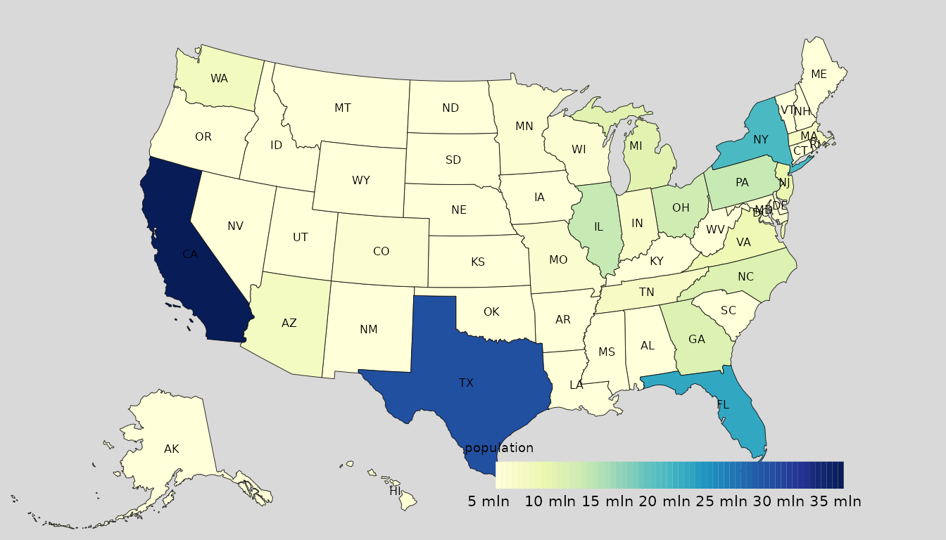
mappingUS(us, var = "population", add_text = "state_id",
          options = mapping.options(nclass = 10, legend.portrait = FALSE))
The facetes argument returns the small multiples, and in
this case, It maps all the divisions.
mappingUS(us, var = "population", aggregation_unit = "division", facets = "division")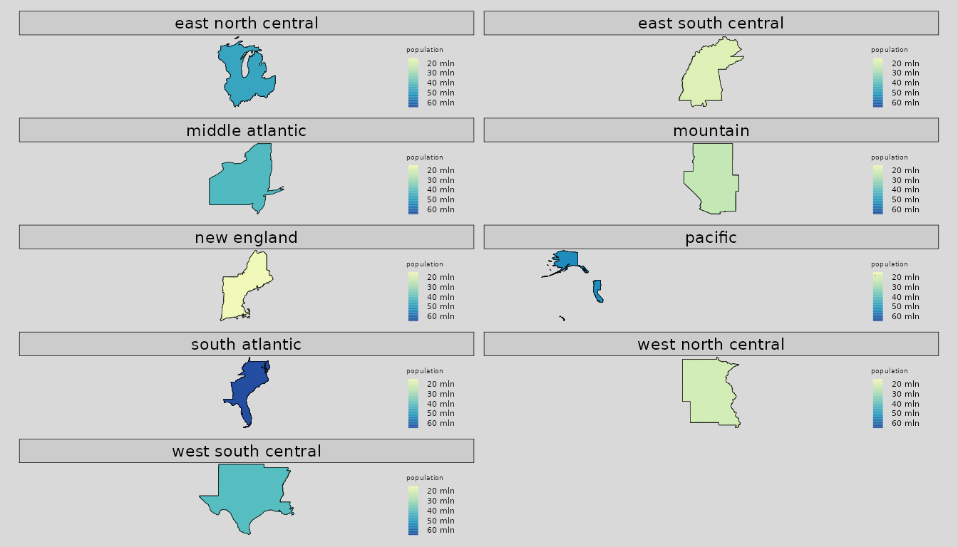
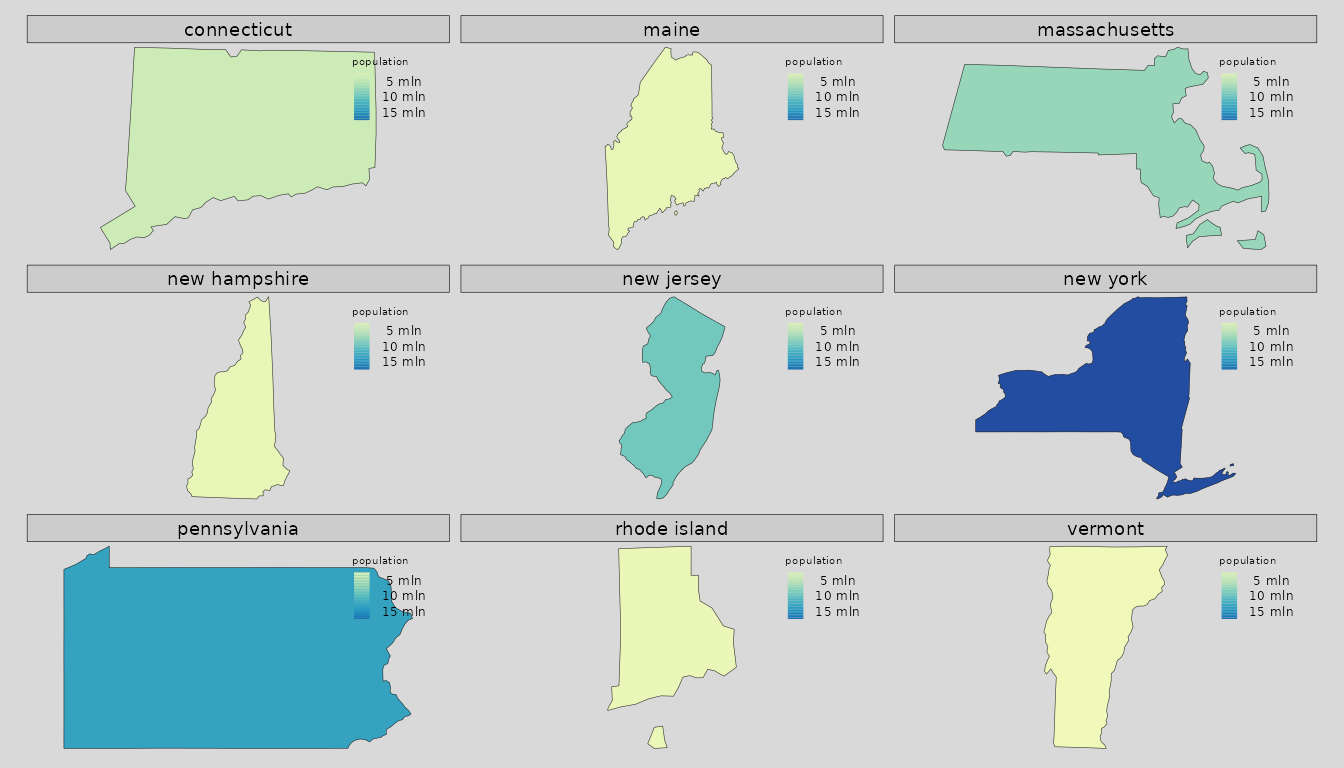
If we are not interested at only the Northeast region, we can apply a subset statement before mapping
Interactive maps
The interactive map functions work as the static functions and they share the same argument.
eu <- EU(data = popEU, unit = "nuts0", colID = "GEO",
         matchWith = "id", check.unit.names = FALSE)
mappingEU(eu, var = "total", type = "interactive")
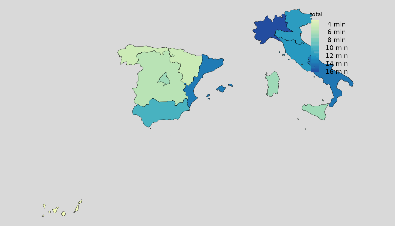
mappingEU(eu, var = "total", type = "interactive",
                      subset = ~I(country == "Spain" | country == "Italy"))
or aggregating for countries (“nuts0”)
mappingEU(eu, var = "total", type = "interactive",
                      aggregation_unit = "nuts0")
Multiple variable will provide a single interactive map with different layers:
and also the facets is implemented for interactive
maps.
A generic mapping() function
The package also provide a generic function to map data,
mapping. This accept object of class sf,
WR, EU, IT, and
US.
library(dplyr)

data("popIT")
popIT <- popIT
coords <- loadCoordIT(unit = "provincia", year = '2019')
cr <- left_join(coords, popIT, by = c( "provincia" = "ID"))
mapping(cr)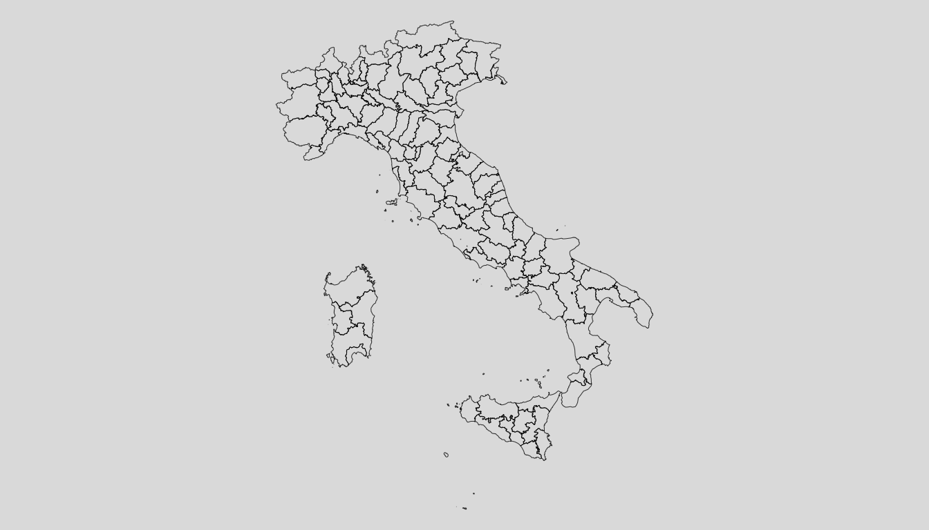
mapping(cr, var = "maschi")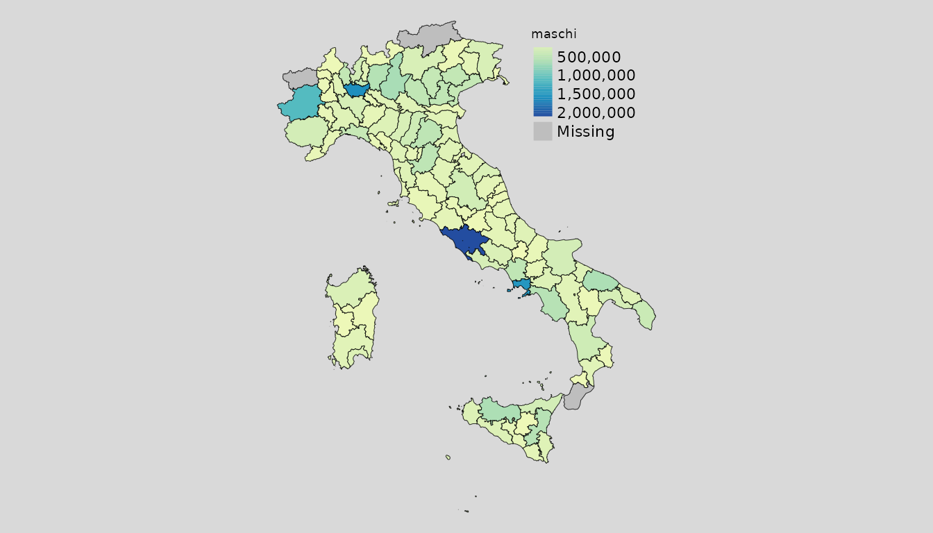
library(sf)
nc = st_read(system.file("shape/nc.shp", package="sf"))
## Reading layer `nc' from data source
##   `/home/runner/work/_temp/Library/sf/shape/nc.shp' using driver `ESRI Shapefile'
## Simple feature collection with 100 features and 14 fields
## Geometry type: MULTIPOLYGON
## Dimension:     XY
## Bounding box:  xmin: -84.32385 ymin: 33.88199 xmax: -75.45698 ymax: 36.58965
## Geodetic CRS:  NAD27
class(nc)
## [1] "sf"         "data.frame"
mapping(nc)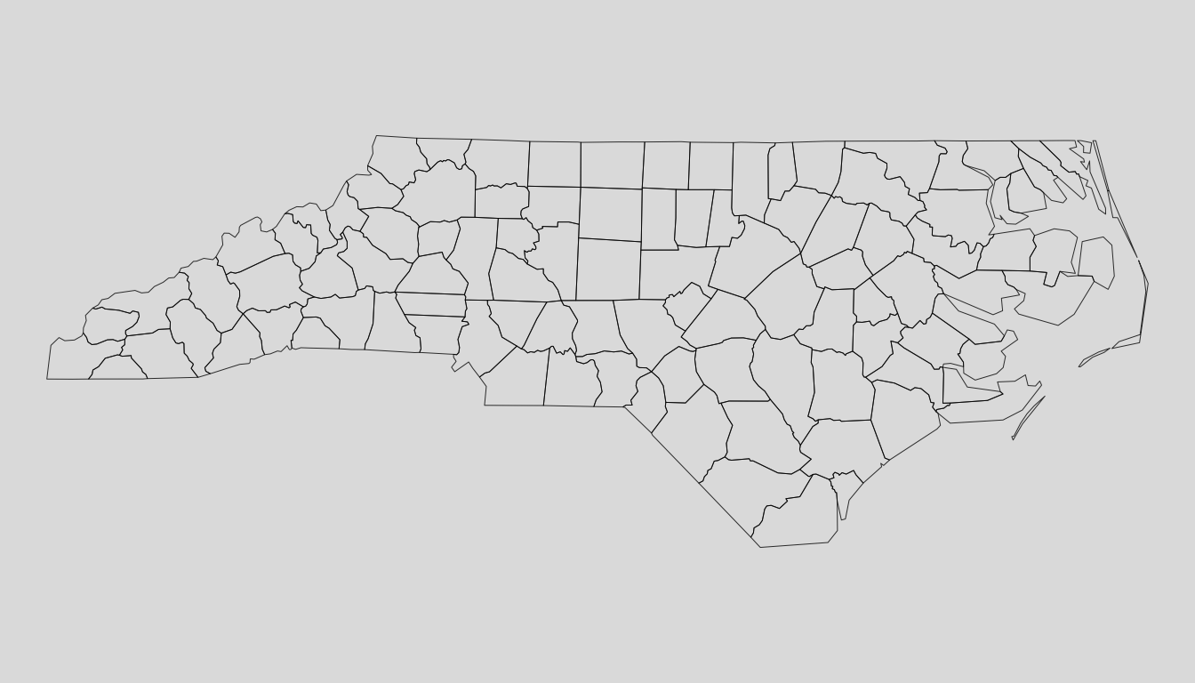
Layout options
Aesthetic options are controlled by mapping.options()
function. General options can be retrieved
single or multiple options may be retrieved
mapping.options("palette.cont")
## [1] "YlGnBu"
mapping.options("legend.position")
## [1] "right" "top"
and we can globally change until a new R session, as follows
mapping.options(legend.position = c("left","bottom"))
mapping.options("legend.position")
## [1] "right" "top"
Options can be changed locally in mapping functions:
map <- mappingEU(eu, var = "total")
map_options <- mappingEU(eu, var = "total",
                         options = mapping.options(list(legend.position = c("left","bottom"),
                                                        title = "EU total population",
                                                        map.frame = FALSE,
                                                        col.style = "pretty")))

library(tmap)
tmap_arrange(map, map_options)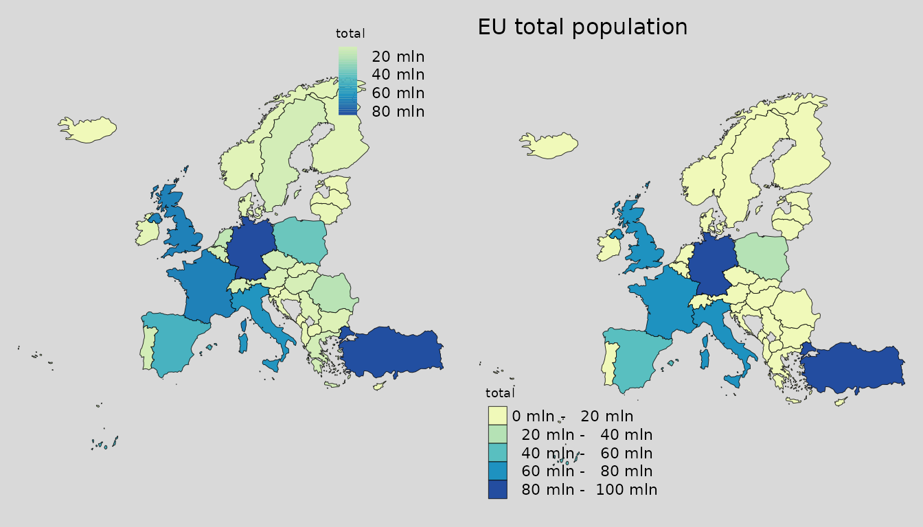
or globally outside the functions. Original options can be reseted
using mapping.options.reset().