mapping using aggregated units
Source:vignettes/mapping-using-aggregated-units.Rmd
mapping-using-aggregated-units.RmdThe CRAN version can be loaded as follows:
or the development version from GitHub:
remotes::install_github('serafinialessio/mapping')The objects created in this package build the hierarchy starting from the statistical units in input to the larger statistical unit aggregate (look at the other vignettes for more details about the hierarchy).
Aggregations arguments allows to easily aggregate and
mapping larger units starting from those given in input.
Italian Examples
data("popIT")
it_pr <- IT(data = popIT, unit = "provincia", year = "2019", check.unit.names = FALSE)
str(it_pr,1)
## Classes 'sf', 'IT', 'IT' and 'data.frame': 107 obs. of 11 variables:
## $ ripartizione : chr "Nord-est" "Sud" "Nord-ovest" "Nord-ovest" ...
## $ regione : chr "Friuli-Venezia Giulia" "Molise" "Piemonte" "Lombardia" ...
## $ code_ripartizione: int 2 4 1 1 1 2 3 4 4 1 ...
## $ code_regione : int 6 14 1 3 3 8 9 18 18 1 ...
## $ code_provincia : int 93 94 96 97 98 99 100 101 102 103 ...
## $ ID : chr "pordenone" "isernia" "biella" "lecco" ...
## $ code : chr "PN" "IS" "BI" "LC" ...
## $ maschi : num 153466 41830 84297 166367 113663 ...
## $ femmine : num 159067 42549 91288 171013 116535 ...
## $ totale : num 312533 84379 175585 337380 230198 ...
## $ geometry :sfc_MULTIPOLYGON of length 107; first list element: List of 1
## ..- attr(*, "class")= chr [1:3] "XY" "MULTIPOLYGON" "sfg"
## - attr(*, "sf_column")= chr "geometry"
## - attr(*, "agr")= Factor w/ 3 levels "constant","aggregate",..: NA NA NA NA NA NA NA NA NA NA
## ..- attr(*, "names")= chr [1:10] "ripartizione" "regione" "code_ripartizione" "code_regione" ...
## - attr(*, "unit")= chr "provincia"
## - attr(*, "year")= chr "2019"
## - attr(*, "colID")= chr "ID"In the structure we have bigger units, as regione
mappingIT(data = it_pr, var = "totale")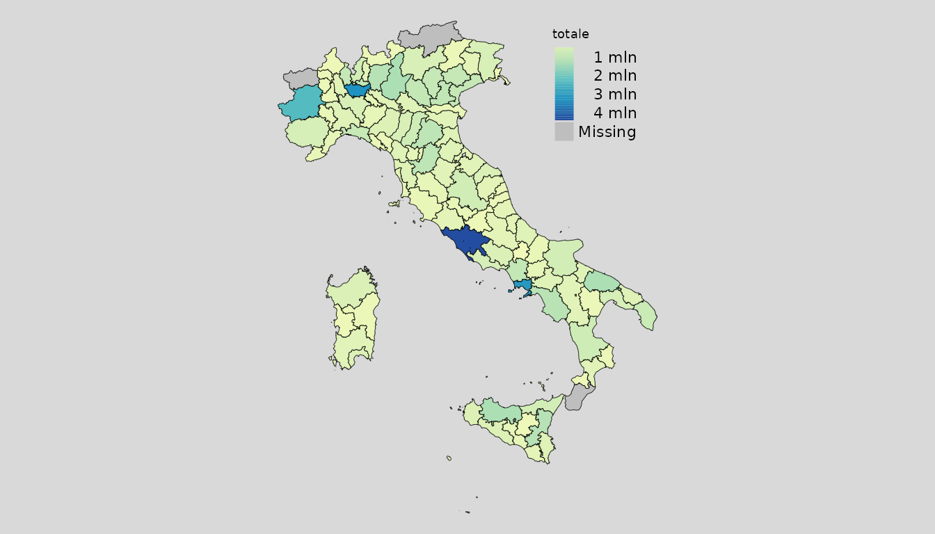
mappingIT(data = it_pr, var = "totale", type = "interactive")Aggregating the province in the beloging regions summing the total population of each province
mappingIT(data = it_pr, var = "totale", aggregation_unit = "regione")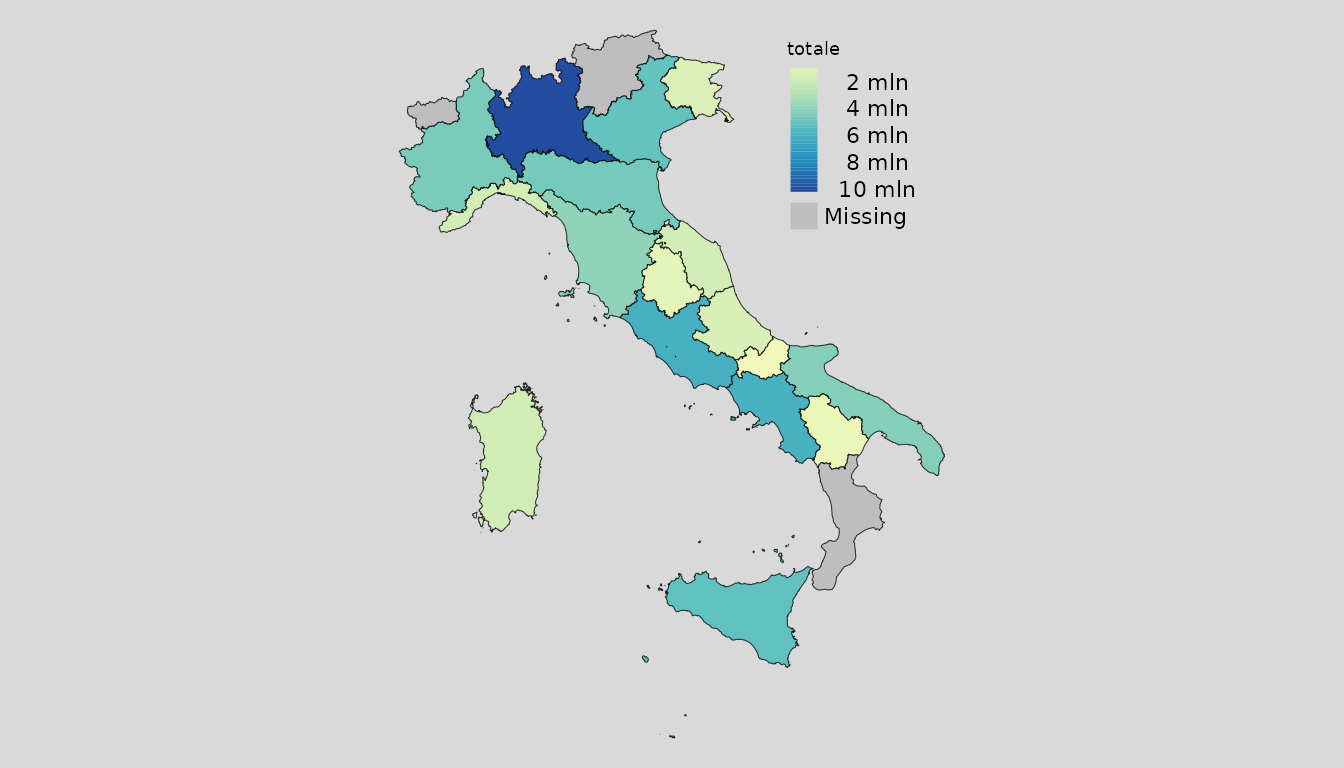
mappingIT(data = it_pr, var = "totale", aggregation_unit = "regione", type = "interactive")or for each ripartizione, removing the missing values
mappingIT(data = it_pr, var = "totale",
aggregation_unit = "ripartizione",
aggregation_fun = function(x) sum(x, na.rm = TRUE))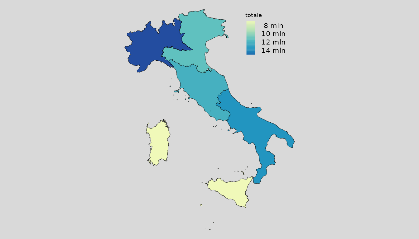
mappingIT(data = it_pr, var = "totale",
aggregation_unit = "ripartizione",
aggregation_fun = function(x) sum(x, na.rm = TRUE),
type = "interactive")This can be also used with facetes
mappingIT(data = it_pr, var = "totale",
aggregation_unit = "regione", facets = "regione")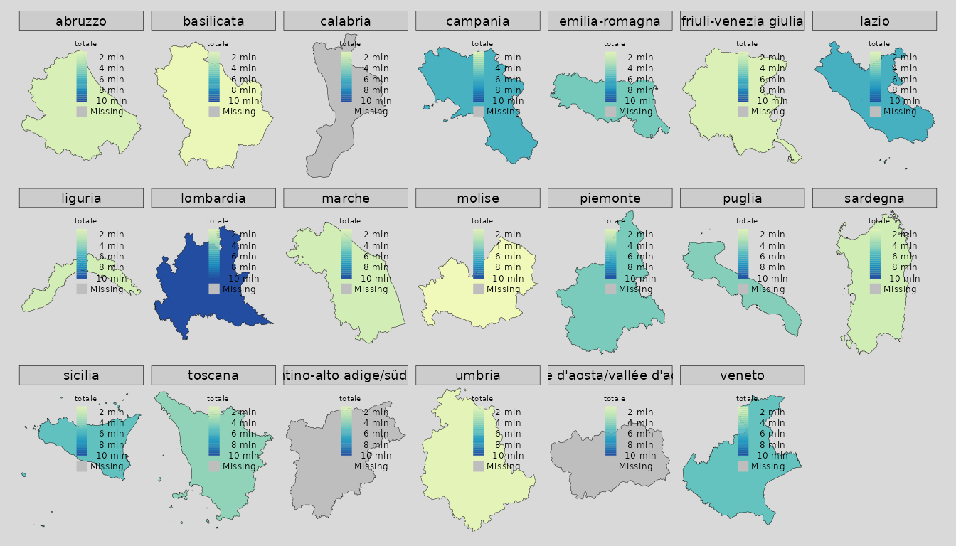
mappingIT(data = it_pr, var = "totale",
aggregation_unit = "regione", facets = "regione",
type = "interactive")
mappingIT(data = it_pr, var = "totale",
aggregation_unit = "ripartizione", facets = "ripartizione",
aggregation_fun = function(x) sum(x, na.rm = TRUE))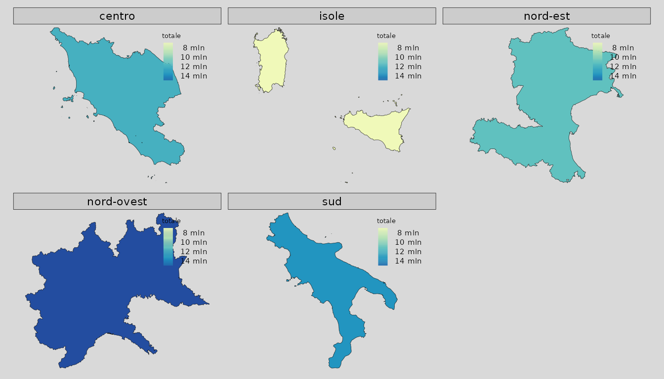
mappingIT(data = it_pr, var = "totale",
aggregation_unit = "ripartizione", facets = "ripartizione",
aggregation_fun = function(x) sum(x, na.rm = TRUE),
type = "interactive")Also in the facetes we can chose the aggregation
mappingIT(data = it_pr, var = "totale",
aggregation_unit = "regione", facets = "ripartizione")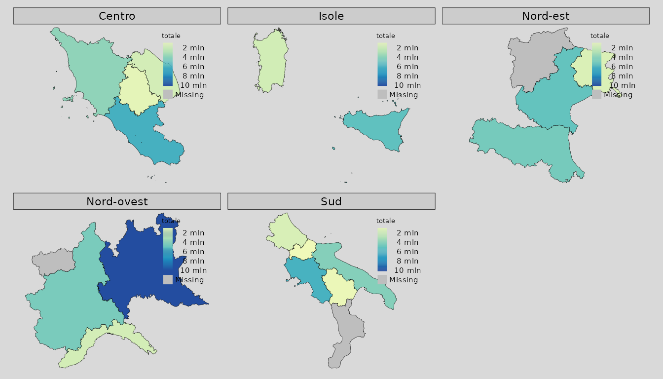
mappingIT(data = it_pr, var = "totale",
aggregation_unit = "regione", facets = "ripartizione",
type = "interactive")European Union Example
data("popEU")
popEU <- popEU
euNuts2 <- EU(data = popEU, colID = "GEO",unit = "nuts2",matchWith = "id")
str(euNuts2,1)
## Classes 'sf', 'EU', 'EU' and 'data.frame': 328 obs. of 16 variables:
## $ GEO : chr "cz05" "cz06" "cz07" "cz08" ...
## $ country : chr "Czechia" "Czechia" "Czechia" "Czechia" ...
## $ iso2 : chr "CZ" "CZ" "CZ" "CZ" ...
## $ iso3 : chr "CZE" "CZE" "CZE" "CZE" ...
## $ country_code: int 203 203 203 203 276 276 276 276 276 276 ...
## $ nuts0_id : chr "CZ" "CZ" "CZ" "CZ" ...
## $ nuts1_id : chr "CZ0" "CZ0" "CZ0" "CZ0" ...
## $ nuts2_id : chr "CZ05" "CZ06" "CZ07" "CZ08" ...
## $ nuts0 : chr "Czechia" "Czechia" "Czechia" "Czechia" ...
## $ nuts1 : chr "Česko" "Česko" "Česko" "Česko" ...
## $ nuts2 : chr "Severovýchod" "Jihovýchod" "Střední Morava" "Moravskoslezsko" ...
## $ TIME : num 2019 2019 2019 2019 2019 ...
## $ total : num 1513693 1696941 1215413 1203299 4143418 ...
## $ male : num 747330 835577 595503 590516 2067094 ...
## $ female : num 766363 861364 619910 612783 2076324 ...
## $ geometry :sfc_MULTIPOLYGON of length 328; first list element: List of 1
## ..- attr(*, "class")= chr [1:3] "XY" "MULTIPOLYGON" "sfg"
## - attr(*, "sf_column")= chr "geometry"
## - attr(*, "agr")= Factor w/ 3 levels "constant","aggregate",..: NA NA NA NA NA NA NA NA NA NA ...
## ..- attr(*, "names")= chr [1:15] "GEO" "country" "iso2" "iso3" ...
## - attr(*, "unit")= chr "nuts2"
## - attr(*, "year")= chr "2021"
## - attr(*, "colID")= chr "GEO"
mappingEU(data = euNuts2, var = "total")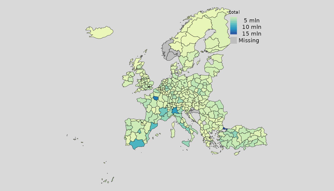
mappingEU(data = euNuts2, var = "total", type = "interactive")Aggregating the nuts 0 in the belonging countries with the average population of each nuts 0
mappingEU(data = euNuts2, var = "total",
aggregation_unit = "nuts0", aggregation_fun = mean)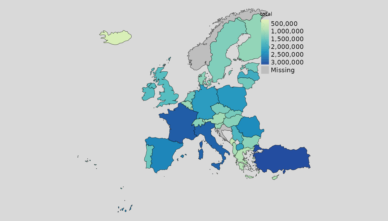
mappingEU(data = euNuts2, var = "total",
aggregation_unit = "nuts0", aggregation_fun = mean,
type = "interactive")or with a summation to have the country population
mappingEU(data = euNuts2, var = "total",
aggregation_unit = "nuts0", aggregation_fun = sum)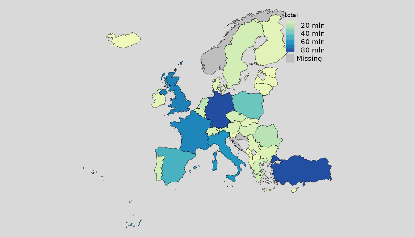
mappingEU(data = euNuts2, var = "total",
aggregation_unit = "nuts0", aggregation_fun = sum,
type = "interactive")We have many countries and the facetes can be visualise well. At this point we can subset, France for example, and show the nuts 1 units.
mappingEU(data = euNuts2, var = "total", subset = ~I(iso3 == "FRA"),
aggregation_unit = "nuts1", aggregation_fun = sum, facets = "nuts1")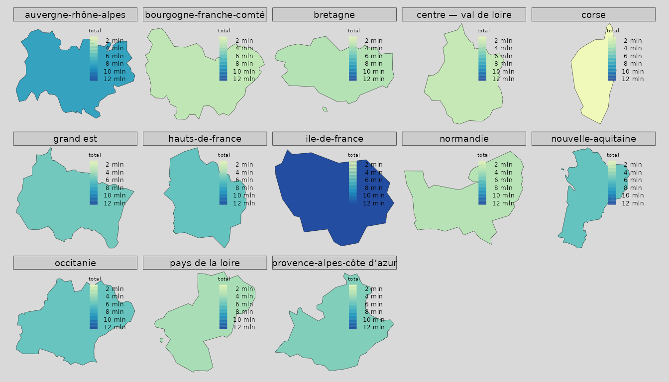
USA Example
data("popUS")
us <- US(data = popUS, unit = "state")
str(us,1)
## Classes 'sf', 'US', 'US' and 'data.frame': 51 obs. of 7 variables:
## $ state_id : chr "MD" "IA" "DE" "OH" ...
## $ id : chr "maryland" "iowa" "delaware" "ohio" ...
## $ state_number: chr "24" "19" "10" "39" ...
## $ region : chr "South" "Midwest" "South" "Midwest" ...
## $ division : chr "South Atlantic" "West North Central" "South Atlantic" "East North Central" ...
## $ population : int 6042718 3156145 967171 11689442 12807060 1929268 7535591 4887871 3013825 2095428 ...
## $ geometry :sfc_MULTIPOLYGON of length 51; first list element: List of 2
## ..- attr(*, "class")= chr [1:3] "XY" "MULTIPOLYGON" "sfg"
## - attr(*, "sf_column")= chr "geometry"
## - attr(*, "agr")= Factor w/ 3 levels "constant","aggregate",..: NA NA NA NA NA NA
## ..- attr(*, "names")= chr [1:6] "state_id" "id" "state_number" "region" ...
## - attr(*, "unit")= chr "state"
## - attr(*, "year")= chr "2018"
## - attr(*, "colID")= chr "id"
mappingUS(data = us, var = "population")
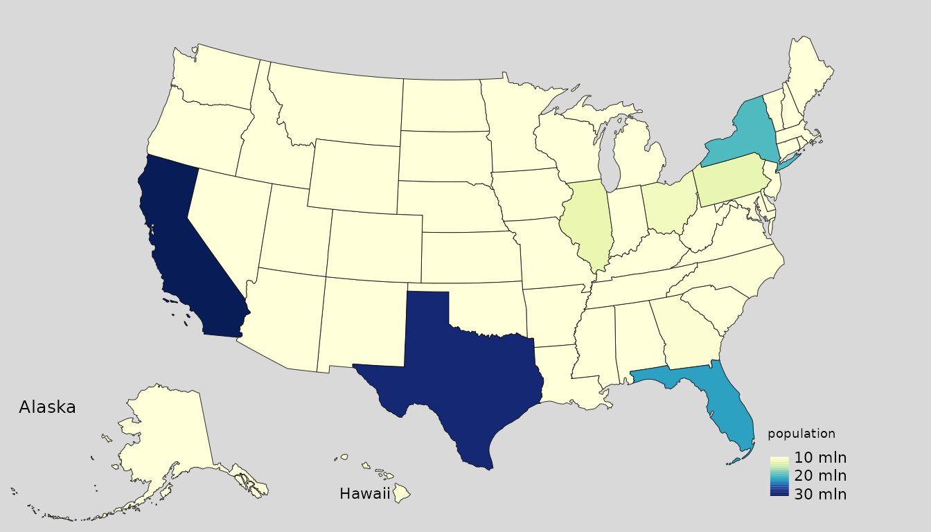
mappingUS(data = us, var = "population", type = "interactive")
mappingUS(data = us, var = "population",
aggregation_unit = "region")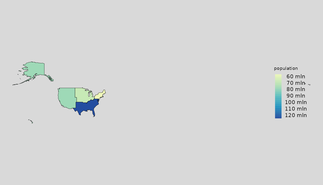
mappingUS(data = us, var = "population",
aggregation_unit = "region",
type = "interactive")
mappingUS(data = us, var = "population",
aggregation_unit = "region", facets = "region")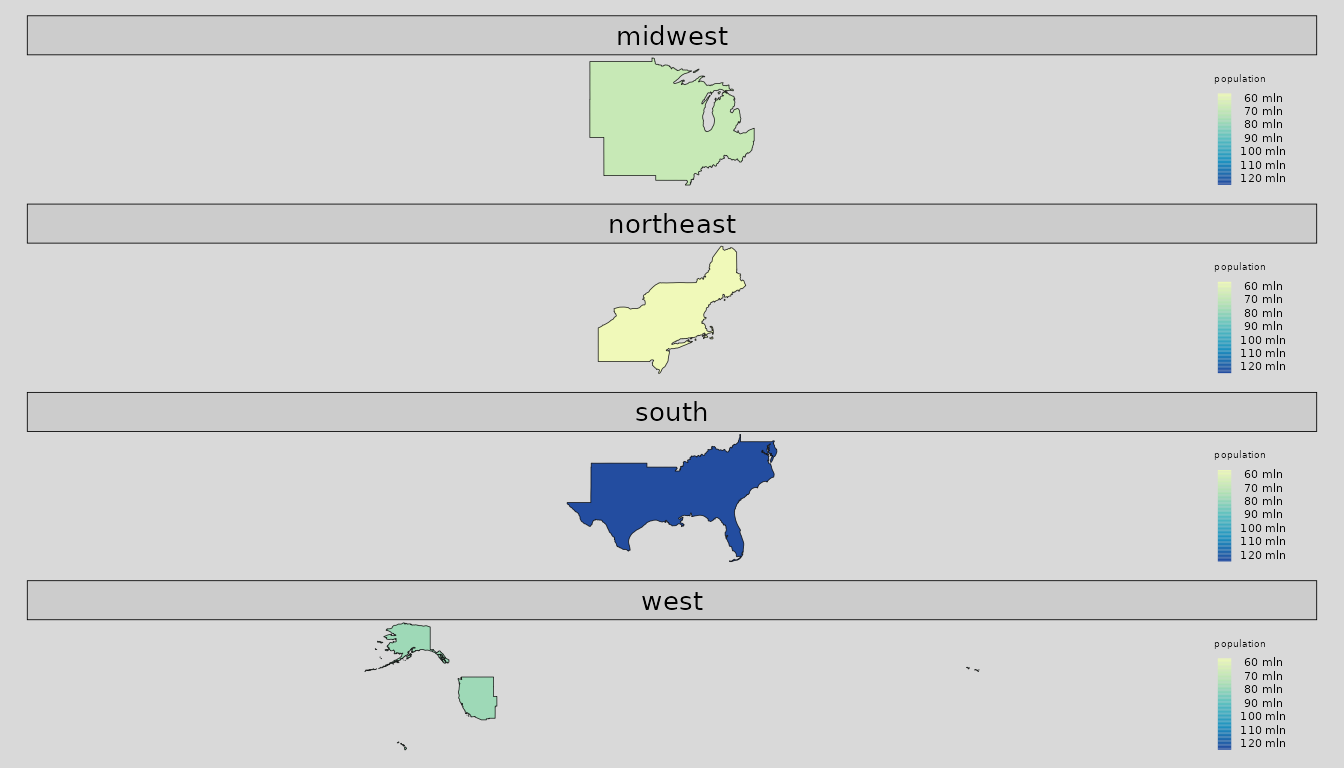
mappingUS(data = us, var = "population",
aggregation_unit = "region", facets = "region",
type = "interactive")World example
data("popWR")
popWR <- popWR
wr <- WR(data = popWR, colID = "country_code",
matchWith = "iso3_eh", check.unit.names = FALSE,
res = "low")
str(wr,1)
## Classes 'sf', 'WR', 'WR' and 'data.frame': 248 obs. of 24 variables:
## $ country_load: chr "Indonesia" "Malaysia" "Chile" "Bolivia" ...
## $ name_formal : chr "Republic of Indonesia" "Malaysia" "Republic of Chile" "Plurinational State of Bolivia" ...
## $ name_wb : chr "Indonesia" "Malaysia" "Chile" "Bolivia" ...
## $ iso2 : chr "ID" "MY" "CL" "BO" ...
## $ iso3 : chr "IDN" "MYS" "CHL" "BOL" ...
## $ country_code: chr "idn" "mys" "chl" "bol" ...
## $ iso3_numeric: chr "360" "458" "152" "068" ...
## $ iso3_un : chr "360" "458" "152" "068" ...
## $ iso2_wb : chr "ID" "MY" "CL" "BO" ...
## $ iso3_wb : chr "IDN" "MYS" "CHL" "BOL" ...
## $ continent : chr "Asia" "Asia" "South America" "South America" ...
## $ region : chr "Asia" "Asia" "Americas" "Americas" ...
## $ subregion : chr "South-Eastern Asia" "South-Eastern Asia" "South America" "South America" ...
## $ region_wb : chr "East Asia & Pacific" "East Asia & Pacific" "Latin America & Caribbean" "Latin America & Caribbean" ...
## $ type : chr "Sovereign country" "Sovereign country" "Sovereign country" "Sovereign country" ...
## $ type_economy: chr "Emerging" "Developing" "Emerging" "Emerging" ...
## $ type_income : chr "Lower middle income" "Upper middle income" "Upper middle income" "Lower middle income" ...
## $ nato : logi FALSE FALSE FALSE FALSE FALSE FALSE ...
## $ ocde : logi FALSE FALSE TRUE FALSE FALSE FALSE ...
## $ country : Factor w/ 265 levels "","Afghanistan",..: 112 150 45 26 193 10 56 111 46 117 ...
## $ total : num 2.68e+08 3.15e+07 1.87e+07 1.14e+07 3.20e+07 ...
## $ male : num 1.35e+08 1.62e+07 9.23e+06 5.70e+06 1.59e+07 ...
## $ female : num 1.33e+08 1.53e+07 9.50e+06 5.65e+06 1.61e+07 ...
## $ geometry :sfc_MULTIPOLYGON of length 248; first list element: List of 178
## ..- attr(*, "class")= chr [1:3] "XY" "MULTIPOLYGON" "sfg"
## - attr(*, "sf_column")= chr "geometry"
## - attr(*, "agr")= Factor w/ 3 levels "constant","aggregate",..: NA NA NA NA NA NA NA NA NA NA ...
## ..- attr(*, "names")= chr [1:23] "country_load" "name_formal" "name_wb" "iso2" ...
## - attr(*, "unit")= chr "country"
## - attr(*, "colID")= chr "country_code"
mappingWR(data = wr, var = "total")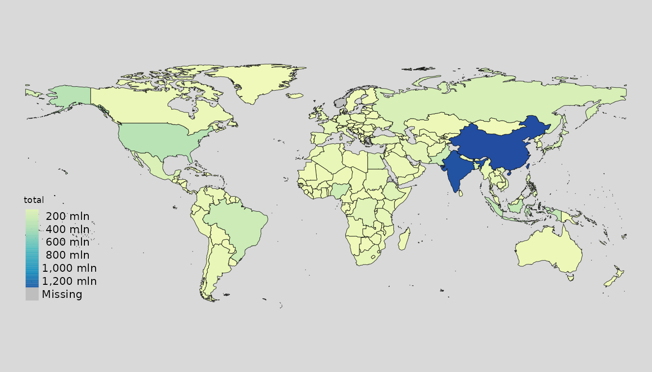
mappingWR(data = wr, var = "total", type = "interactive")Aggregating by continent
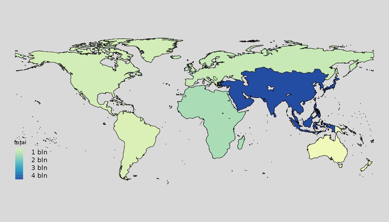
mappingWR(data = wr, var = "total",
aggregation_unit = "continent",
aggregation_fun = function(x) sum(x, na.rm = TRUE))